Forcing and orbit

Select an SSP or RCP scenario

CMIP6

Control is possible through the namelist file fort.4. Inside you will find the namelist NAERAD, which contains the options for CMIP5 and CMIP6 greenhouse gas forcing. To activate CMIP6 forcing set the logic switch LCMIP6 = .true.. When NCMIPFIXYR is set to a value >0, it is interpreted as a fix forcing year. In the example below we use constant 1850 GHG forcing. If NCMIPFIXYR=0 the actual model year is used, and forcing changes from year to year. Note, that only greenhouse gases and solar radiation are set through this namelist.

The recommended way to ensure the namelist changes are made conistently, is to use the add_namelist_changes from esm-tools.

&NAERAD
   LCMIP6 = .true.
   CMIP6DATADIR = 'PATH_TO_CMIP6_POOL'
   NCMIPFIXYR = 1850
   SSPNAME = 'historical'

Historic forcing is available for the years 1850 to 2014.

&NAERAD
   LCMIP6 = .true.
   CMIP6DATADIR = 'PATH_TO_CMIP6_POOL'
   NCMIPFIXYR = 0
   SSPNAME = 'historical'

Available SSPs are: SSP1-1.9, SSP1-2.6, SSP2-4.5, SSP3-7.0, SSP3-LowNTCF, SSP4-3.4, SSP4-6.0, SSP4-6.0, SSP5-3.4-OS, SSP5-8.5. Covered years are 2015 to 2100.

&NAERAD
   LCMIP6 = .true.
   CMIP6DATADIR = 'PATH_TO_CMIP6_POOL'
   NCMIPFIXYR = 0
   SSPNAME = 'SSP3-7.0'

The model also supports one percent increase per year and sudden four times incease of CO2 experiments through the additional logic switches L1PCTCO2 and LA4XCO2. The base value from which the the increase starts is set via NCMIPFIXYR.

For a multiple of the reference concentration other than those two fixed cases, set LANXCO2 and give the factor in RNXCO2. That is the usual way to specify a time slice whose CO2 is not a whole number of doublings.

&NAERAD
   LCMIP6 = .true.
   CMIP6DATADIR = 'PATH_TO_CMIP6_POOL'
   NCMIPFIXYR = 1850
   SSPNAME = 'historical'
   L1PCTCO2 = 'true'

For a more detailed look at the use of these forcing consult the source code file src/ifs/climate/updrgas.F90

CMIP5

Control is analogous to CMIP6 but we use LCMIP5, CMIP5DATADIR, and NRCP instead. Avaiable RCP are:

SELECT CASE (NRCP)
CASE (0)
  FILENAME='ghg_histo.txt'
CASE (1)
  FILENAME='ghg_rcp3PD.txt'
CASE (2)
  FILENAME='ghg_rcp45.txt'
CASE (3)
  FILENAME='ghg_rcp60.txt'
CASE (4)
  FILENAME='ghg_rcp85.txt'

For a more detailed look at the use of these forcing consult the source code file src/ifs/climate/updrgas.F90

Supply your own greenhouse gas time series

Applies to: everything except AWI-ESM3-cc, where CO2 is a prognostic tracer and is not read from a concentration file at all.

There is no namelist entry that takes a filename. OpenIFS builds the name it wants from the scenario switch and the simulation year, and then looks for exactly that name. So a custom series is not a setting, it is a file you put where the model will look, under the name the model will construct.

The recipe is the same for all three CMIP generations. Copy the pool directory somewhere you can write, replace the values in the file for the gas and years you care about, and point the data directory at your copy:

oifs:
    add_namelist_changes:
        fort.4:
            NAERAD:
                CMIP6DATADIR: '/work/<project>/<user>/input/my-cmip6-data'

Leave the file names alone. Renaming a file is the one thing that cannot work, because the model is not reading a name you gave it.

What differs is which switch drives the name and what you are editing:

• CMIP5, driven by NRCP, cy43r3 only. Plain text, one row per year, columns YEAR CO2 CH4 N2O CFC11 CFC12. Edit it in any editor. The names are fixed: ghg_histo.txt for the historical case, and ghg_rcp3PD.txt, ghg_rcp45.txt, ghg_rcp60.txt or ghg_rcp85.txt for the RCPs.

• CMIP6, driven by SSPNAME, both cycles. One NetCDF per gas, holding mole_fraction_of_<gas>_in_air(time, sector). Sector 0 is global, 1 is the northern hemisphere and 2 the southern, and all three are read, so change all three unless you actually want a hemispheric gradient.

• CMIP7, driven by SCENARIONAME, cy48r1 only. One NetCDF per gas, global mean only, so the variable is simply co2(time), ch4(time) and so on. These sit under <CMIP7DATADIR>/ghg/ScenarioMIP/ rather than directly in the data directory.

For the NetCDF cases the edit itself is one command. To scale a series, or to write your own values in from a text file:

ncap2 -s 'co2 = co2 * 2.0' co2_in.nc co2_out.nc
ncap2 -s 'mole_fraction_of_carbon_dioxide_in_air(:,0) = 400.0' co2_in.nc co2_out.nc

Check that the model used it

Almost nothing checks this for you, so check the file before you submit. ncdump -v co2 yourfile.nc | tail costs a second and catches the case where you edited the wrong gas, the wrong sector or the wrong years.

Afterwards, grep NODE.001_01 for ECE_CMIP_GHG. It prints the full path of the file it opened and the concentration it took out of it:

ECE_CMIP_GHG: Set JYEAR=MIN(JYEAR,2022)=        1850
/work/<project>/<user>/input/oifs-48r1/cmip-data//ghg/co2_input4MIPs_GHGConcentrations_CMIP_CR-CMIP-1-0-0_gm_1750-2022.nc
ZZ_YEARS=   182.5000
ZZCO2=   284.2973

The path is the check that matters. If it is not your directory, the namelist change did not take, and ZZCO2 then tells you which value the run is actually using.

The one thing the model does catch is a name it cannot find, and it does so at startup rather than silently falling back:

ECE_CMIP_GHG: No such file or directory

A scenario name that does not exist fails the same way:

ECE_CMIP_GHG : unknown CMIP6 scenario

Wrong values in a file with the right name abort nothing. The run starts, finishes and is wrong, which is why the two checks above are worth the minute they cost.

Control Aerosol Scaling

Applies to: AWI-CM3 v3.2 through v3.3.1 only. Before v3.2 it is not implemented, which has the same effect as deactivating it, and from v3.4.0 onwards the anthropogenic aerosol forcing comes from MACv2-SP instead, so none of this applies there.

It is controlled via the fort.4 namelist parameter NAERANT_SCALE in the NAERAD namelist. By default it is set to 1 (activated). If activated, the default aerosol levels (which have an annual cycle that does not change over the years) are scaled according to the spatio-temporal field given in ifsdata/aerosol_scale_1850_2085_r2005.nc. This is supposed to model the anthropogenic influence on aerosol levels over time. For running paleo-simulations one might want to deactivate this. This is best done via an entry in the esm-tools runscript:

oifs:
    add_namelist_changes:
        fort.4:
            NAERAD:
                NAERANT_SCALE: 0

For a more detailed look, consult the source code files, e.g. src/ifs/phys_ec/su_aer_scalefactor.F90

Control orbital parameters

The orbital parameters (eccentricity, obliquity, and longitude of perihelion) can be controlled through the namelist NAMORB inside the fort.4 file. For details of the implementation, consider looking at yomorb.F90 and su0phy.F90. Controllable orbital parameters are turned on with the logic switch: LCORBMD=true, which is turned off by default. There are then three modes with which the orbital parameters can be controlled.

• Under ORBMODE=variable_year mode the orbital parameters are calculated according to Berger et al. 1978 for the current year of the simulation. This is the default. The calculation can be considered reliable within ~+-1 million years of the present.

• Under ORBMODE=fixed_year mode the orbital parameters are calculated according to Berger et al. 1978 for the fixed year set by the namelist variable ORBIY. If you choose fixed year but set no year, the default is 1950.

• Under fixed_parameters you have manual control over the parameters ORBECCEN, ORBOBLIQ and ORBMVELP. If you choose fixed parameters but set no parameters, the default ones are for 1950.

ORBMVELP is the longitude of perihelion measured from the moving vernal equinox, in degrees. That is the convention PMIP publishes in, so PMIP values go in unchanged and a mid-Holocene run takes 0.87.

The model adds the 180 degrees itself, in yomorb.F90, where mvelpp = (mvelp + 180.0)*degrad turns what you set into the internal ORBMVELPP, so do not add it yourself. Both examples below are vernal equinox values: 102.7 for 1950, and 275.41 for the PMIP4 last interglacial.

Example for manual control:

&NAMORB
   LCORBMD = true
   ORBMODE = 'fixed_parameters'
   ORBECCEN = 0.016715
   ORBOBLIQ = 23.4441
   ORBMVELP = 102.7

In order to have esm-tools create an openIFS namelist of that form one can adjust the simulation YAML. The following example would let openIFS compute top of the atmosphere insolation based on an LIG orbit whose parameters are as defined for PMIP4:

oifs:
    add_namelist_changes:
        fort.4:
            NAMORB:
                LCORBMD: TRUE
                ORBMODE: 'fixed_parameters'
                ORBECCEN: 0.039378
                ORBOBLIQ: 24.040
                ORBMVELP: 275.41

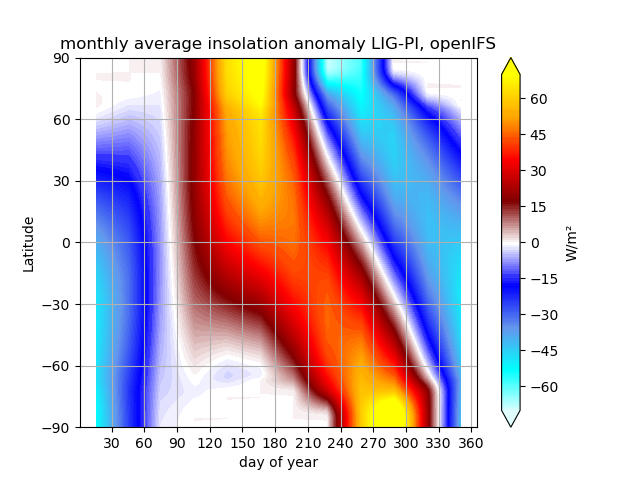
The resulting anomaly of top of the atmosphere insolation shows the expected anomalies across latitudes over time:

Accelerate the orbit

variable_year advances the orbit exactly one year per model year, and NAMORB has no acceleration factor, so an accelerated orbit is not something you switch on. What you do instead is hold the orbit fixed within a leg and step it between legs, which works because esm_tools rewrites fort.4 for every leg:

oifs:
    orb_year_0: -9000        # orbital year at the start of the experiment
    orb_accel: 10            # orbital years per model year
    add_namelist_changes:
        fort.4:
            NAMORB:
                LCORBMD: true
                ORBMODE: 'fixed_year'
                ORBIY: "$(( ${oifs.orb_year_0} + (${start_date!year} - ${general.initial_date!year}) * ${oifs.orb_accel} ))"

OpenIFS then computes the Berger 1978 parameters for that year itself, which is the same solution variable_year would have used. The orbit is constant inside a leg and jumps at each leg boundary, so keep the legs short enough that the jump stays smaller than the signal you are looking for.

Deriving the year from the dates rather than from ${general.run_number} matters, because then a restart or a change of leg length does not shift the orbit under you.

Every leg prints a MODULE YOMORB block into NODE.001_01 giving ORBMODE, the ORBIY it used, and the eccentricity, obliquity and perihelion derived from it. Compare ORBIY between two consecutive legs, because that is the one thing worth checking: if it has not moved, the orbit is not stepping and every leg is running the same one.

This has been checked in configuration only. The namelist comes out right, ORBIY = -9000 on the first leg and -8900 ten model years later at an acceleration of ten, but no production run has used it yet.

Comparison of PI (1850) insolation for various relevant models

Differences between ECHAM6 and openIFS generated insolation can be deemed negligibly small. There is an overall offset of both ECHAM6 and openIFS with respect to the insolation computed from the PMIP4 PI orbit settings - that question may deserve further investigation. Note that ECHAM6 computes their modern insolation based on an internal orbit solution, i.e. the orbital parameters are never explicitly provided to the model as a forcing.

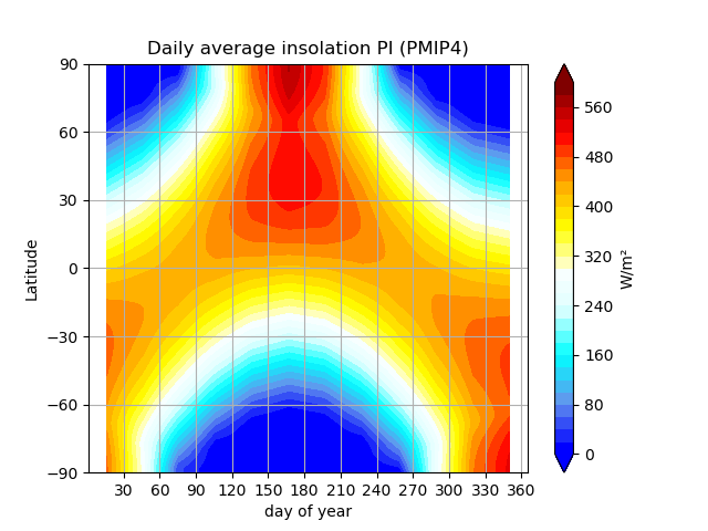
Insolation based on PMIP4 orbital parameters, computed based on climlab.

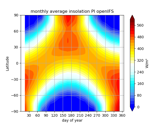
OpenIFS computed PI insolation, monthly means.

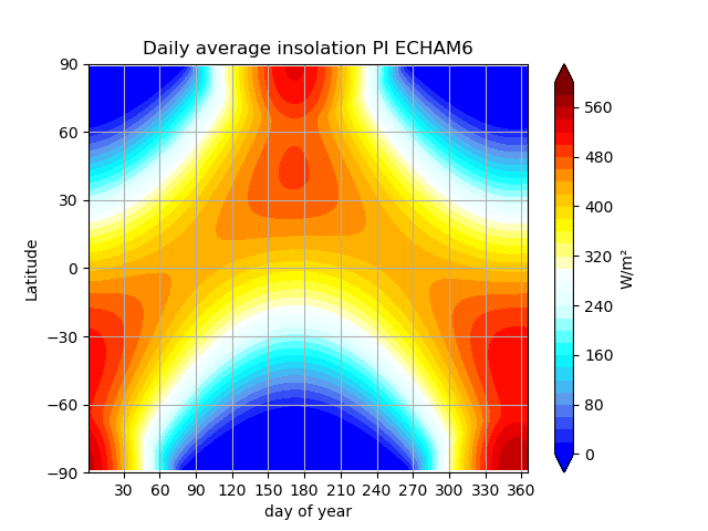
ECHAM6 computed PI insolation, daily means.

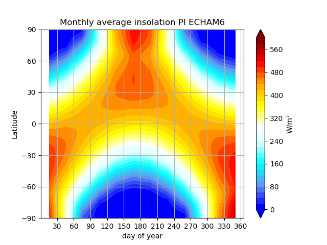
ECHAM6 computed PI insolation, monthly means, interpolated to openIFS grid.

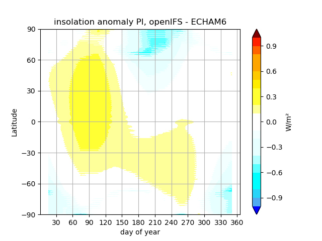
Anomaly of PI insolation, openIFS minus ECHAM6.

Files towards generation of the plots above are available in source/releases/3.1/.